ceres-solver tutorial
ceres-solver tutorial 문서를 공부한 글입니다.
dependency
# CMake
sudo apt-get install cmake
# google-glog + gflags
sudo apt-get install libgoogle-glog-dev libgflags-dev
# BLAS & LAPACK
sudo apt-get install libatlas-base-dev
# Eigen3
sudo apt-get install libeigen3-dev
# SuiteSparse and CXSparse (optional)
sudo apt-get install libsuitesparse-dev
ceres-solver installation
cd catkin_ws/src
git clone https://ceres-solver.googlesource.com/ceres-solver
// git clone 받은 디렉토리 옆에 ceres-bin 생성
mkdir ceres-bin
cd ceres-bin
make -j3
make test
make install
Introduction
\[min \frac{1}{2}\sum_{i}\rho(||f_{i}(x_{i_{1}},\cdots,x_{i_{k}})||^{2})\]Ceres는 $x_{j}$가 어떤 범위 안에 있을 때 non-linear least square 문제를 풀 수 있게 해준다.
\[\rho(||f_{i}(x_{i_{1}},\cdots,x_{i_{k}})||^{2})\]이 ResidualBlock이고, $f_{i}(\cdot)$이 CostFunction,이다. 또한 $x_{i}$ 값들의 집합을 ParameterBlock이라고 한다. $\rho_{i}$는 LossFunction이다.
특별한 케이스로 $\rho_{i}(x)=x$, x값의 범위는 $-infty$ 부터 $infty$까지로 설정한다. 그러면 식을
\[\frac{1}{2}\sum_{i}||f_{i}(x_{i_{1}},\cdots,x_{i_{k}})||^{2}\]로 간단하게 나타낼 수 있다.
Hello world!
cd ceres-bin/bin
//실행
./helloworld
코드는 ceres-solver/examples/helloworld.cc를 보면 된다.
ceres-solver에서 가장 간단한 예제인 Hello wolrd를 통해 $\frac{1}{2}(10-x)^{2}$ 를 최소로 만드는 x값을 구해보자. 우리는 쉽게 x가 10일 때 이 값이 최소가 되는것을 알 수 있지만 이 예제로 ceres의 기본을 배워보자.
struct CostFunctor {
  template <typename T>
  bool operator()(const T* const x, T* residual) const {
    residual[0] = 10.0 - x[0];
    return true;
  }
};
cost function $f(x)=10-x$로 설정하는 부분이다. template을 써서 어떤 input과 output이 들어오던 T 형태로 받게 된다. residual 값이 double일수도 있고, vector 형태일수도 있기 때문이다.
int main(int argc, char** argv) {
  google::InitGoogleLogging(argv[0]);

  // The variable to solve for with its initial value. It will be
  // mutated in place by the solver.
  double x = 0.5;
  const double initial_x = x;
initial_x 값을 0.5로 설정한다.
  // Build the problem.
  Problem problem;

  // Set up the only cost function (also known as residual). This uses
  // auto-differentiation to obtain the derivative (jacobian).
  CostFunction* cost_function =
      new AutoDiffCostFunction<CostFunctor, 1, 1>(new CostFunctor);
  problem.AddResidualBlock(cost_function, nullptr, &x);
Problem을 선언하고, cost_function에 AutoDiffCostFunction을 통해 미분을 해준다. 만약 residual에 여러 값이 있다면 T=Jet으로 jacobian을 나타내게 된다.
이 cost_function을 ResidualBlock에 넣어 풀게 되면,
  // Run the solver!
  Solver::Options options;
  options.minimizer_progress_to_stdout = true;
  Solver::Summary summary;
  Solve(options, &problem, &summary);

  std::cout << summary.BriefReport() << "\n";
  std::cout << "x : " << initial_x << " -> " << x << "\n";
  return 0;
}

iteration 2번만에 x값이 10이 나오는 것을 볼 수 있다.
Powell’s Function
cd ceres-bin/bin
./powell

| 위와 같이 cost function이 있다고 할 때, $\frac{1}{2} | F(x) | ^2$ 를 최소화 하는 x를 찾아보자. |
struct F1 {
  template <typename T>
  bool operator()(const T* const x1, const T* const x2, T* residual) const {
    // f1 = x1 + 10 * x2;
    residual[0] = x1[0] + 10.0 * x2[0];
    return true;
  }
};

struct F2 {
  template <typename T>
  bool operator()(const T* const x3, const T* const x4, T* residual) const {
    // f2 = sqrt(5) (x3 - x4)
    residual[0] = sqrt(5.0) * (x3[0] - x4[0]);
    return true;
  }
};

struct F3 {
  template <typename T>
  bool operator()(const T* const x2, const T* const x3, T* residual) const {
    // f3 = (x2 - 2 x3)^2
    residual[0] = (x2[0] - 2.0 * x3[0]) * (x2[0] - 2.0 * x3[0]);
    return true;
  }
};

struct F4 {
  template <typename T>
  bool operator()(const T* const x1, const T* const x4, T* residual) const {
    // f4 = sqrt(10) (x1 - x4)^2
    residual[0] = sqrt(10.0) * (x1[0] - x4[0]) * (x1[0] - x4[0]);
    return true;
  }
};
위처럼 각 residual을 정의해주고,
double x1 =  3.0; double x2 = -1.0; double x3 =  0.0; double x4 = 1.0;

Problem problem;

// Add residual terms to the problem using the using the autodiff
// wrapper to get the derivatives automatically.
problem.AddResidualBlock(
  new AutoDiffCostFunction<F1, 1, 1, 1>(new F1), nullptr, &x1, &x2);
problem.AddResidualBlock(
  new AutoDiffCostFunction<F2, 1, 1, 1>(new F2), nullptr, &x3, &x4);
problem.AddResidualBlock(
  new AutoDiffCostFunction<F3, 1, 1, 1>(new F3), nullptr, &x2, &x3)
problem.AddResidualBlock(
  new AutoDiffCostFunction<F4, 1, 1, 1>(new F4), nullptr, &x1, &x4);
초기값 설정해준 뒤, ResidualBlock에 넣어준다.
Initial x1 = 3, x2 = -1, x3 = 0, x4 = 1
iter      cost      cost_change  |gradient|   |step|    tr_ratio  tr_radius  ls_iter  iter_time  total_time
   0  1.075000e+02    0.00e+00    1.55e+02   0.00e+00   0.00e+00  1.00e+04       0    4.95e-04    2.30e-03
   1  5.036190e+00    1.02e+02    2.00e+01   2.16e+00   9.53e-01  3.00e+04       1    4.39e-05    2.40e-03
   2  3.148168e-01    4.72e+00    2.50e+00   6.23e-01   9.37e-01  9.00e+04       1    9.06e-06    2.43e-03
   3  1.967760e-02    2.95e-01    3.13e-01   3.08e-01   9.37e-01  2.70e+05       1    8.11e-06    2.45e-03
   4  1.229900e-03    1.84e-02    3.91e-02   1.54e-01   9.37e-01  8.10e+05       1    6.91e-06    2.48e-03
   5  7.687123e-05    1.15e-03    4.89e-03   7.69e-02   9.37e-01  2.43e+06       1    7.87e-06    2.50e-03
   6  4.804625e-06    7.21e-05    6.11e-04   3.85e-02   9.37e-01  7.29e+06       1    5.96e-06    2.52e-03
   7  3.003028e-07    4.50e-06    7.64e-05   1.92e-02   9.37e-01  2.19e+07       1    5.96e-06    2.55e-03
   8  1.877006e-08    2.82e-07    9.54e-06   9.62e-03   9.37e-01  6.56e+07       1    5.96e-06    2.57e-03
   9  1.173223e-09    1.76e-08    1.19e-06   4.81e-03   9.37e-01  1.97e+08       1    7.87e-06    2.60e-03
  10  7.333425e-11    1.10e-09    1.49e-07   2.40e-03   9.37e-01  5.90e+08       1    6.20e-06    2.63e-03
  11  4.584044e-12    6.88e-11    1.86e-08   1.20e-03   9.37e-01  1.77e+09       1    6.91e-06    2.65e-03
  12  2.865573e-13    4.30e-12    2.33e-09   6.02e-04   9.37e-01  5.31e+09       1    5.96e-06    2.67e-03
  13  1.791438e-14    2.69e-13    2.91e-10   3.01e-04   9.37e-01  1.59e+10       1    7.15e-06    2.69e-03

Ceres Solver v1.12.0 Solve Report
----------------------------------
                                     Original                  Reduced
Parameter blocks                            4                        4
Parameters                                  4                        4
Residual blocks                             4                        4
Residual                                    4                        4

Minimizer                        TRUST_REGION

Dense linear algebra library            EIGEN
Trust region strategy     LEVENBERG_MARQUARDT

                                        Given                     Used
Linear solver                        DENSE_QR                 DENSE_QR
Threads                                     1                        1
Linear solver threads                       1                        1

Cost:
Initial                          1.075000e+02
Final                            1.791438e-14
Change                           1.075000e+02

Minimizer iterations                       14
Successful steps                           14
Unsuccessful steps                          0

Time (in seconds):
Preprocessor                            0.002

  Residual evaluation                   0.000
  Jacobian evaluation                   0.000
  Linear solver                         0.000
Minimizer                               0.001

Postprocessor                           0.000
Total                                   0.005

Termination:                      CONVERGENCE (Gradient tolerance reached. Gradient max norm: 3.642190e-11 <= 1.000000e-10)

Final x1 = 0.000292189, x2 = -2.92189e-05, x3 = 4.79511e-05, x4 = 4.79511e-05
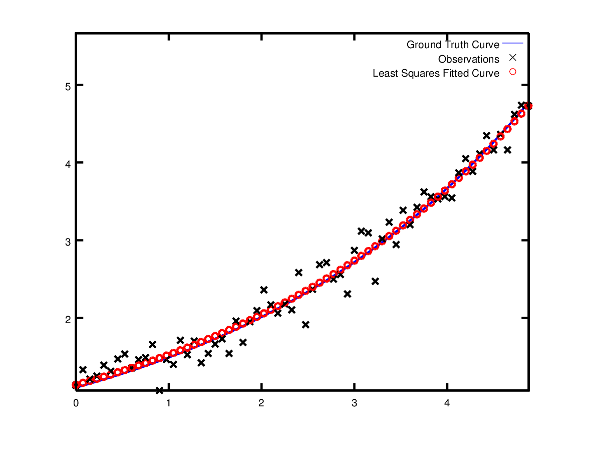
Curve Fitting
위에서는 간단한 optimization을 해보았다면, 이제 실제 데이터를 가지고 curve를 fitting하는 예제를 풀어보자.
\[y=e^{0.3x+0.1}, \sigma=0.2\]$\sigma$는 Gaussian noise
위의 curve를 만들기 위해 $y=e^{mx+c}$라는 모델을 가정하자.
const double data[] = {
  0.000000e+00, 1.133898e+00,
  7.500000e-02, 1.334902e+00,
  1.500000e-01, 1.213546e+00,
  2.250000e-01, 1.252016e+00,
  3.000000e-01, 1.392265e+00,
  3.750000e-01, 1.314458e+00,
  4.500000e-01, 1.472541e+00,
  5.250000e-01, 1.536218e+00,
  6.000000e-01, 1.355679e+00,
  6.750000e-01, 1.463566e+00,
넣어줄 데이터의 x,y 값이 쭈르륵 있다. x는 0.075씩 증가하고, y값은
// Data generated using the following octave code.
//   randn('seed', 23497);
//   m = 0.3;
//   c = 0.1;
//   x=[0:0.075:5];
//   y = exp(m * x + c);
//   noise = randn(size(x)) * 0.2;
//   y_observed = y + noise;
//   data = [x', y_observed'];
다음 식으로 랜덤값을 가지도록 설정한다.
struct ExponentialResidual {
  ExponentialResidual(double x, double y)
      : x_(x), y_(y) {}

  template <typename T>
  bool operator()(const T* const m, const T* const c, T* residual) const {
    residual[0] = y_ - exp(m[0] * x_ + c[0]);
    return true;
  }

 private:
  // Observations for a sample.
  const double x_;
  const double y_;
};
ExponentialResidual을 위와 같이 정의한다.
실제관측된 y_ 값에서 가정한 모델 $e^{m[0]x_+c[0]}$을 빼서 이 값들의 합이 최소가 되는
m,c를 찾는 것이 목표이다.
double m = 0.0;
double c = 0.0;

Problem problem;
for (int i = 0; i < kNumObservations; ++i) {
  CostFunction* cost_function =
       new AutoDiffCostFunction<ExponentialResidual, 1, 1, 1>(
           new ExponentialResidual(data[2 * i], data[2 * i + 1]));
  problem.AddResidualBlock(cost_function, nullptr, &m, &c);
}
위에 있는 넣어줄 데이터를 형태를 맞춰서 x,y값을 data[2*i], data[2*i+1]로 설정해주었다.
iter      cost      cost_change  |gradient|   |step|    tr_ratio  tr_radius  ls_iter  iter_time  total_time
   0  1.211734e+02    0.00e+00    3.61e+02   0.00e+00   0.00e+00  1.00e+04       0    5.34e-04    2.56e-03
   1  1.211734e+02   -2.21e+03    0.00e+00   7.52e-01  -1.87e+01  5.00e+03       1    4.29e-05    3.25e-03
   2  1.211734e+02   -2.21e+03    0.00e+00   7.51e-01  -1.86e+01  1.25e+03       1    1.10e-05    3.28e-03
   3  1.211734e+02   -2.19e+03    0.00e+00   7.48e-01  -1.85e+01  1.56e+02       1    1.41e-05    3.31e-03
   4  1.211734e+02   -2.02e+03    0.00e+00   7.22e-01  -1.70e+01  9.77e+00       1    1.00e-05    3.34e-03
   5  1.211734e+02   -7.34e+02    0.00e+00   5.78e-01  -6.32e+00  3.05e-01       1    1.00e-05    3.36e-03
   6  3.306595e+01    8.81e+01    4.10e+02   3.18e-01   1.37e+00  9.16e-01       1    2.79e-05    3.41e-03
   7  6.426770e+00    2.66e+01    1.81e+02   1.29e-01   1.10e+00  2.75e+00       1    2.10e-05    3.45e-03
   8  3.344546e+00    3.08e+00    5.51e+01   3.05e-02   1.03e+00  8.24e+00       1    2.10e-05    3.48e-03
   9  1.987485e+00    1.36e+00    2.33e+01   8.87e-02   9.94e-01  2.47e+01       1    2.10e-05    3.52e-03
  10  1.211585e+00    7.76e-01    8.22e+00   1.05e-01   9.89e-01  7.42e+01       1    2.10e-05    3.56e-03
  11  1.063265e+00    1.48e-01    1.44e+00   6.06e-02   9.97e-01  2.22e+02       1    2.60e-05    3.61e-03
  12  1.056795e+00    6.47e-03    1.18e-01   1.47e-02   1.00e+00  6.67e+02       1    2.10e-05    3.64e-03
  13  1.056751e+00    4.39e-05    3.79e-03   1.28e-03   1.00e+00  2.00e+03       1    2.10e-05    3.68e-03
Ceres Solver Report: Iterations: 13, Initial cost: 1.211734e+02, Final cost: 1.056751e+00, Termination: CONVERGENCE
Initial m: 0 c: 0
Final   m: 0.291861 c: 0.131439
Simple bundle adjuster
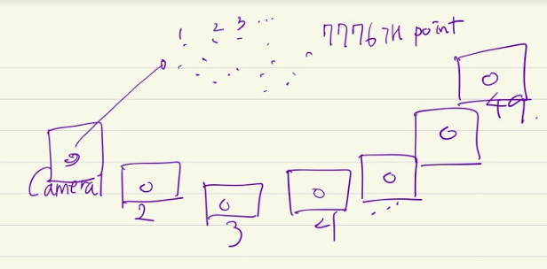
BA는 reprojection error를 최소화 시키기 위해 3D point position과 카메라 parameter들을 adjustment하는 것이다.

reprojection error란, 맵 상의 3차원 포인트들을 키프레임 이미지에 투영 시킨 위치와 해당 영상 프레임에서 실제 관측된 위치 차이를 말한다. 이 차이를 최소화 시키는게 BA가 하는 일이다. 카메라 parameter는 extrinsic parameter, intrinsic parameter 두 종류가 있다.
BA example을 돌리기 위해 BAL dataset을 이용한다. 여기서

다음 데이터셋중 하나를 받아서
./simple_bundle_adjuster /경로/txt파일
을 해주면 실행 된다.
gleefe1995@gleefe1995-desktop:~/ceres_ws/src/ceres-bin/bin$ ./simple_bundle_adjuster /home/gleefe1995/ceres_ws/src/ceres-bin/dataset/problem-21-11315-pre.txt
iter      cost      cost_change  |gradient|   |step|    tr_ratio  tr_radius  ls_iter  iter_time  total_time
   0  4.413239e+06    0.00e+00    8.63e+07   0.00e+00   0.00e+00  1.00e+04        0    2.08e-02    5.28e-02
   1  3.542514e+04    4.38e+06    2.40e+06   1.86e+02   9.99e-01  3.00e+04        1    4.46e-02    9.75e-02
   2  3.118098e+04    4.24e+03    8.60e+05   1.38e+02   8.90e-01  5.71e+04        1    4.13e-02    1.39e-01
   3  3.051581e+04    6.65e+02    1.76e+05   6.77e+01   9.64e-01  1.71e+05        1    4.08e-02    1.80e-01
   4  3.042415e+04    9.17e+01    1.48e+05   4.56e+01   9.23e-01  4.36e+05        1    4.28e-02    2.22e-01
   5  3.038873e+04    3.54e+01    9.38e+04   5.79e+01   8.99e-01  8.88e+05        1    4.18e-02    2.64e-01
   6  3.037939e+04    9.34e+00    2.38e+04   2.97e+01   9.69e-01  2.66e+06        1    4.17e-02    3.06e-01
   7  3.037865e+04    7.45e-01    2.66e+03   9.91e+00   9.94e-01  7.99e+06        1    4.26e-02    3.49e-01

Solver Summary (v 2.0.0-eigen-(3.3.4)-lapack-suitesparse-(5.1.2)-cxsparse-(3.1.9)-eigensparse-no_openmp)

                                     Original                  Reduced
Parameter blocks                        11336                    11336
Parameters                              34134                    34134
Residual blocks                         36455                    36455
Residuals                               72910                    72910

Minimizer                        TRUST_REGION

Dense linear algebra library            EIGEN
Trust region strategy     LEVENBERG_MARQUARDT

                                        Given                     Used
Linear solver                     DENSE_SCHUR              DENSE_SCHUR
Threads                                     1                        1
Linear solver ordering              AUTOMATIC                 11315,21
Schur structure                         2,3,9                    2,3,9

Cost:
Initial                          4.413239e+06
Final                            3.037865e+04
Change                           4.382861e+06

Minimizer iterations                        8
Successful steps                            8
Unsuccessful steps                          0

Time (in seconds):
Preprocessor                         0.031990

  Residual only evaluation           0.034258 (8)
  Jacobian & residual evaluation     0.133728 (8)
  Linear solver                      0.134065 (8)
Minimizer                            0.340961

Postprocessor                        0.000913
Total                                0.373865

Termination:                      CONVERGENCE (Function tolerance reached. |cost_change|/cost: 3.371144e-07 <= 1.000000e-06)
BAL problem의 각 residual은 3차원 포인트와 9개의 camera parameter에 depend한다. 3개는 rodrigue’s axis-angle vector, 3개는 translation, 1개는 focal length, 2개는 radial distortion이다.
data format은 다음과 같다.
<num_cameras> <num_points> <num_observations>
<camera_index_1> <point_index_1> <x_1> <y_1>
…
<camera_index_num_observations> <point_index_num_observations> <x_num_observations>
<y_num_observations>
<camera_1> … <camera_num_cameras>
<point_1> … <point_num_points>

observation 데이터개수, camera pose 데이터개수, 3D point 데이터개수
num_observation + 9*num_cameras + 3*num_points 하면 전체 데이터개수가 나온다.
camera pose는 camera[0~2] -> angle-axis rotation, camera[3~5] -> translation, camera[6] -> focal length, camera[7,8] -> radial distortion이다.
// Read a Bundle Adjustment in the Large dataset.
class BALProblem {
 public:
  ~BALProblem() {
    delete[] point_index_;
    delete[] camera_index_;
    delete[] observations_;
    delete[] parameters_;
  }

  int num_observations() const { return num_observations_; }
  const double* observations() const { return observations_; }
  double* mutable_cameras() { return parameters_; }
  double* mutable_points() { return parameters_ + 9 * num_cameras_; }

  double* mutable_camera_for_observation(int i) {
    return mutable_cameras() + camera_index_[i] * 9;
  }
  double* mutable_point_for_observation(int i) {
    return mutable_points() + point_index_[i] * 3;
  }

  bool LoadFile(const char* filename) {
    FILE* fptr = fopen(filename, "r");
    if (fptr == NULL) {
      return false;
    };

    FscanfOrDie(fptr, "%d", &num_cameras_);
    FscanfOrDie(fptr, "%d", &num_points_);
    FscanfOrDie(fptr, "%d", &num_observations_);

    point_index_ = new int[num_observations_];
    camera_index_ = new int[num_observations_];
    observations_ = new double[2 * num_observations_];

    num_parameters_ = 9 * num_cameras_ + 3 * num_points_;
    parameters_ = new double[num_parameters_];

    for (int i = 0; i < num_observations_; ++i) {
      FscanfOrDie(fptr, "%d", camera_index_ + i);
      FscanfOrDie(fptr, "%d", point_index_ + i);
      for (int j = 0; j < 2; ++j) {
        FscanfOrDie(fptr, "%lf", observations_ + 2 * i + j);
      }
    }

    for (int i = 0; i < num_parameters_; ++i) {
      FscanfOrDie(fptr, "%lf", parameters_ + i);
    }
    return true;
  }

 private:
  template <typename T>
  void FscanfOrDie(FILE* fptr, const char* format, T* value) {
    int num_scanned = fscanf(fptr, format, value);
    if (num_scanned != 1) {
      LOG(FATAL) << "Invalid UW data file.";
    }
  }

  int num_cameras_;
  int num_points_;
  int num_observations_;
  int num_parameters_;

  int* point_index_;
  int* camera_index_;
  double* observations_;
  double* parameters_;
};
이 txt파일을 BALProblem에서 불러온다.
struct SnavelyReprojectionError {
  SnavelyReprojectionError(double observed_x, double observed_y)
      : observed_x(observed_x), observed_y(observed_y) {}

  template <typename T>
  bool operator()(const T* const camera,
                  const T* const point,
                  T* residuals) const {
    // camera[0,1,2] 회전 행렬
    T p[3];
    ceres::AngleAxisRotatePoint(camera, point, p);
    // camera[3,4,5] 는 tranlation
    p[0] += camera[3]; p[1] += camera[4]; p[2] += camera[5];

    // Compute the center of distortion. The sign change comes from
    // the camera model that Noah Snavely's Bundler assumes, whereby
    // the camera coordinate system has a negative z axis.
    // camera coordinate가 negative z axis를 갖고 있어서 -를 붙여주는 것 같다.
    T xp = - p[0] / p[2];
    T yp = - p[1] / p[2];

    // Apply second and fourth order radial distortion.
    // distortion을 고려
    const T& l1 = camera[7];
    const T& l2 = camera[8];
    T r2 = xp*xp + yp*yp;
    T distortion = 1.0 + r2  * (l1 + l2  * r2);

    // Compute final projected point position.
    // 위에서 계산한 focal, distortion, xp, yp를 가지고 예측된 x,y값을 계산
    const T& focal = camera[6];
    T predicted_x = focal * distortion * xp;
    T predicted_y = focal * distortion * yp;

    // The error is the difference between the predicted and observed position.
    // 예측값과 실제 관측된 값의 차이 = error
    residuals[0] = predicted_x - T(observed_x);
    residuals[1] = predicted_y - T(observed_y);
    return true;
  }

   // Factory to hide the construction of the CostFunction object from
   // the client code.
   static ceres::CostFunction* Create(const double observed_x,
                                      const double observed_y) {
     return (new ceres::AutoDiffCostFunction<SnavelyReprojectionError, 2, 9, 3>(
                 new SnavelyReprojectionError(observed_x, observed_y)));
   }

  double observed_x;
  double observed_y;
};
predicted_x,y : 3D point in world coordinate -> 2D point in camera coordinates (투영된 점)
observed_x,y : 실제 관측된 점
이 두 개의 점의 x,y좌표의 차이를 뺀 것을 residual[0], [1]에 저장한다.
 // Create residuals for each observation in the bundle adjustment problem. The
  // parameters for cameras and points are added automatically.
  ceres::Problem problem;
  for (int i = 0; i < bal_problem.num_observations(); ++i) {
    // Each Residual block takes a point and a camera as input and outputs a 2
    // dimensional residual. Internally, the cost function stores the observed
    // image location and compares the reprojection against the observation.

    ceres::CostFunction* cost_function = SnavelyReprojectionError::Create(
        observations[2 * i + 0], observations[2 * i + 1]);
    problem.AddResidualBlock(cost_function,
                             NULL /* squared loss */,
                             bal_problem.mutable_camera_for_observation(i),
                             bal_problem.mutable_point_for_observation(i));
  }
위와같이 나타낼 수 있다. curve fitting example이랑 비슷한 부분이 많다.
pose graph 2d
실행방법
여기에서 2d pose graph optimization 데이터셋 하나를 받고
cd ceres-bin/bin
./pose_graph_2d --input /home/gleefe1995/Downloads/input_M3500_g2o.g2o
plot
python3 plot_results.py --optimized_poses ./poses_optimized.txt --initial_poses ./poses_original.txt
matplotlib를 설치하라고 하면
sudo pip3 install matplotlib
파이썬3로 실행했기 때문에 pip3로 설치했다.

참조
http://ceres-solver.org/nnls_tutorial.html#hello-world